DS 3000 - Summer 2020
DS Report
Identifying Patterns in Plant Growth
Yevhen Horban, Pranav Ahluwalia
Executive Summary:
This project is focused on identifying the patterns and predicting the number of roses produced in a specific greenhouse based on the conditions inside and outside of the greenhouse. Plants usually need nutritious soil, water, sunlight, and carbon dioxide to grow. While the greenhouse controls the constant supply of nutrition and water, other conditions are variable. The amount of how much roses are produced appears to have a sinusoidal pattern with a variable vertical shift, amplitude, and period that depend on weather conditions.
Outline
1. INTRODUCTION
Problem Statement
In our project, we analyze the effects of different environmental factors on the number of roses a specific greenhouse produces. This project assumes that if the environment were controlled, then the production of flowers would follow a sinusoidal pattern with no noise. Since the climate is not controlled, it is our objective to explore the relationship between its changes and the shift in the pattern of production.
Significance of the Problem
The nature of this particular business is such that the flowers are often sold before they are produced, and it is necessary to know ahead of time how much produce to sell. Also, at times when the peaks of the production curves of different flowers align the freezers that preserve flowers before they are sold run out of the room and the lifespan of the flowers that are left in the room temperature shortens. Tackling this problem matters because if a company knows the amount of product it is going to produce, it can plan for accommodating the storage and adjust prices if necessary to maximize its profit.
Questions/Hypothesis
Given the problem and its importance, as mentioned earlier, we set out to tackle the following questions:
- Is there a linear relationship between the weather conditions and the number of flowers produced? If not, what is the relationship?
- Is there an accumulative or delayed effect of the weather conditions on the dependent variable? What is it?
- Is there a pattern in the number of flowers produced? What periods appear to be more stable or have less noise in the number of flowers produced? What parts of the natural cycle (amplitude, period, vertical shift) are affected by the weather?
- Is there a relationship between the weather conditions and the deviation from the natural production cycle? Which features are the most influential on the deviations of the cycle?
- Is there a linear or nonlinear regression model that can predict the number of flowers produced? Which one is more accurate?
- How do the features correlate with each other? Can we reduce their number to make the prediction model more accurate?
Hypotheses:
- Hypothesis about features:
- Null: The quantity of the flowers produced and the selected weather features have no relationship
- Alternative: The number of flowers produced and the selected weather features have a relationship
- Hypothesis about machine learning algorithms:
- Null: Linear regression IS the best predictor of the quantity of the flowers produced based on the weather features.
- Alternative: Linear regression IS NOT the best predictor of the quantity of the flowers produced based on the weather features.
- Hypothesis about additional features on regression models:
- Null: Mathematically manipulated features WILL NOT change the accuracy of the models.
- Alternative: Mathematically manipulated features WILL change the accuracy of the models.
2. METHOD
2.1. Data Acquisition
We obtained our time-series data from the company that owns the greenhouse and combined it with the historical weather data from Weather Underground to get 1036 by 18 data set. We are going to use the daily averages of the amount of sunlight, the number of minutes the lamps were turned on, the amount of CO2, the temperature inside and outside, dew point, humidity, and atmospheric pressure to predict the number of flowers produced on the given date using regression.
https://www.wunderground.com/history/monthly/ua/brovary/UKBB
import pandas as pd

url_org_data = 'https://raw.githubusercontent.com/h0rban/flower-harvest-prediction/master/data/redeagle.csv'
df = pd.read_csv(url_org_data)
df
2.2. Variables
Rsum is in lux
Pressure is in Hg
Lamps are in minutes
Humidity is in percent
Temperatures are in ºC
CO2 in parts per million
Independent Variables (feature variables)
inside of the greenhouse:
    - lux of sun
    - temperature
    - concentration of CO2
    - minutes the lamps were turned on

minimum, maximum, and average outside of the greenhouse:
    - temperature
    - dew point
    - humidity
    - pressure
Dependent Variables (target variable)
quantity of flowers produced
Rationale
Our features are all the independent variables listed above. They are already continuous, numerical data points and do not require feature engineering with them. Our target variable is the number of flowers produced, which is also a continuous numerical value and a target variable for a regression model. However, we will try to modify both features and the target variable to reduce noise and explore possible relationships.
2.3. Data Analysis
Predictive Model
We will predict the number of flowers produced the following day, given the weather conditions. These predictors are significant because flowers are living creatures that respond to their environment. In addition to the features described above, we are going to mathematically manipulate the data to explore some of our questions and hypothesis.
A Supervised Learning Problem
Since will are seeking to obtain a continuous output variable, this is a supervised regression problem.
Machine Learning Algorithms to be Applied
We will be using Multiple Linear, Ridge, Lasso, kNN, Bayesian Ridge, KernelRidge, and Gaussian Process regression algorithms because it is not clear whether they will be accurate predictors of the number of flowers produced. We expect Bayesian Ridge, KernelRidge, and Gaussian Process regression algorithms work the best because the examples in the scikit learn documentation suggests that they are good at predicting sinusoidal data.
3. RESULTS
df.dropna(inplace = True)
Process variables
Convert string representation of date to Date object
df['Date'] = pd.to_datetime(df['Date'], format='%m/%d/%y')
Data Wrangling
Select features and target form the dataframe
features = df.drop(['Date', 'Produced'], axis = 1)
features
target = df['Produced']
target
Feature extraction
There might not be a linear relationship between features and the target variable, so we use a polynomial feature extraction technique to explore nonlinear relationships in our predictive models.
from sklearn.preprocessing import PolynomialFeatures

# returns a data frame that contains polynomials from 2 to the given degree of the given features
def features_to_poly(features, degrees):
    poly_feature_dfs = []
    for feature in features.columns:
        values = features[feature]
        poly = PolynomialFeatures(degree = degrees, include_bias = False) # we tried using interaction_only = False but it did not work for some reason
        feature_poly = poly.fit_transform(values.values.reshape(-1,1))
        feature_df = pd.DataFrame(feature_poly, columns = [feature + '^' + str(index) for index in range(1, degrees + 1)])
        poly_feature_dfs.append(feature_df.drop(feature + '^' + str(1), axis = 1))
    return pd.concat(poly_feature_dfs, axis = 1)


features_poly = features_to_poly(features, 10)
features_poly
One of the questions we are exploring in this project is whether the weather features have a delayed or an accumulating effect on the target variable. Hence, we will use a feature extraction techniques to generate additional features to explore hidden relationships in our data.
import statistics as st

# returns the given values after applying a given function to the given number of moving values
# this allows to use moving average, range and other functions by ignoring the missing vaules on the edges
def n_moving_func(values, n, func):
    out = []
    length = len(values)
    for index in range(0, length):
        s = index - n // 2
        e = index + n // 2 + 1
        if s < 0:
            s = 0
        if e >= length:
            e = length
        out.append(func(values[s : e]))
    return out


# returns the given values after applying a given function to the given number of previous values
# this allows to sum, or find the range and other functions by ignoring the missing values in the begining
def n_prev_func(values, n, func):
    out = []
    for index in range(0, len(values)):
        s = index - n + 1
        if s < 0:
            s = 0
            temp = values[s : index + 1]
            temp.append(values[index])
            out.append(func(temp))
        else:
            out.append(func(values[s : index + 1]))
    return out


# returns the derivative of given values
# the first value will be the same as the second
def df_dt(values):
    out = [values[1] - values[0]]
    for index in range(1, len(values)):
        out.append(values[index] - values[index - 1])
    return out


# returns linked relatives of the given values
# the first value and dividing by zero will result in a 1
def link_r(values):
    out = [1]
    for index in range(1, len(values)):
        out.append(1) if values[index - 1] == 0 else out.append(values[index] / values[index - 1])
    return out


# returns the range of the given values
def get_range(values):
    return max(values) - min(values)


# returns a dataframe with the result of applying every given function to every column in the given dataframe
def apply_func_to_df(dataframe, funcs, include_original = False):
    new_df = pd.DataFrame()
    for feature in dataframe.columns:
        if include_original:
            new_df[feature] = dataframe[feature]
        for name, func in funcs.items():
            new_df[feature + '_' + name] = pd.Series(func(dataframe[feature]))
    return new_df


# functions that are going to applied to the features
dd_and_lr = {'dd': df_dt, 'lr' : link_r}
funcs = {'3_moving_mean': lambda values: n_moving_func(values, 3, st.mean),
         '5_moving_mean': lambda values: n_moving_func(values, 5, st.mean),
         '7_moving_mean': lambda values: n_moving_func(values, 7, st.mean),
         '3_moving_sd': lambda values: n_moving_func(values, 3, st.stdev),
         '5_moving_sd': lambda values: n_moving_func(values, 5, st.stdev),
         '7_moving_sd': lambda values: n_moving_func(values, 7, st.stdev),
         '3_prev_sum': lambda values: n_prev_func(values.tolist(), 3, sum),
         '7_prev_sum': lambda values: n_prev_func(values.tolist(), 7, sum),
         '21_prev_sum': lambda values: n_prev_func(values.tolist(), 21, sum),
         '3_prev_sd': lambda values: n_prev_func(values.tolist(), 3, st.stdev),
         '7_prev_sd': lambda values: n_prev_func(values.tolist(), 7, st.stdev),
         '21_prev_sd': lambda values: n_prev_func(values.tolist(), 21, st.stdev),
         '3_prev_range': lambda values: n_prev_func(values.tolist(), 3, get_range),
         '7_prev_range': lambda values: n_prev_func(values.tolist(), 7, get_range),
         '21_prev_range': lambda values: n_prev_func(values.tolist(), 21, get_range)}

# this will take a while
features_additional =  apply_func_to_df(apply_func_to_df(features, funcs), dd_and_lr, include_original = True)
features_additional
The following line combines the resulting data frames of feature extraction into a one. Also, add a day number column to two of the data frames (it turned out to be significant to the models)
features_combined = pd.concat([features, apply_func_to_df(features, dd_and_lr), features_poly, features_additional], axis = 1)

features['DayNum'] = df.index
features_combined['DayNum'] = df.index

features_combined
Target Extraction
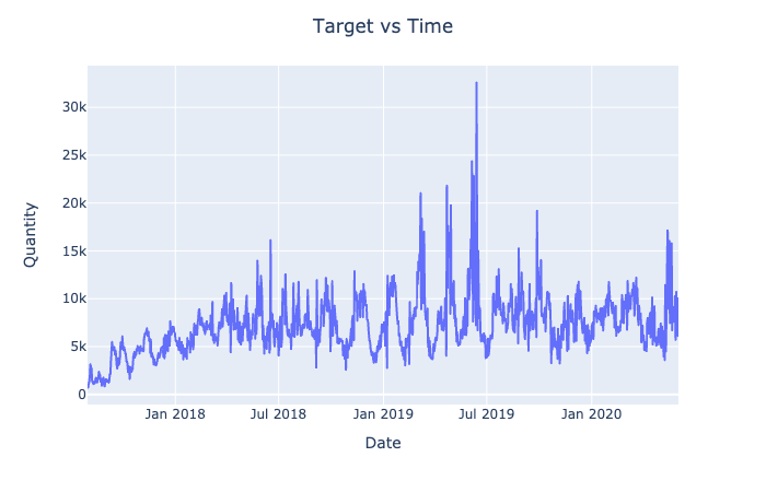
The data for the target variable may be too noisy for the prediction algorithms to identify the pattern. Hence, we will explore the possibilities of smoothening the target variable.
Please see these links for scatterplots:
import plotly.express as px
target = df['Produced']
px.line(df, x = 'Date', y = target)\
.update_layout(title = "Target vs Time",
title_x = 0.5,
yaxis_title = "Quantity").show()
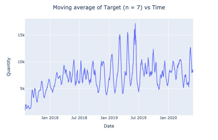
px.line(df, x = 'Date', y = n_moving_func(target.tolist(), 7, st.mean))\
.update_layout(title = "Moving average of Target (n = 7) vs Time",
title_x = 0.5,
yaxis_title = "Quantity").show()
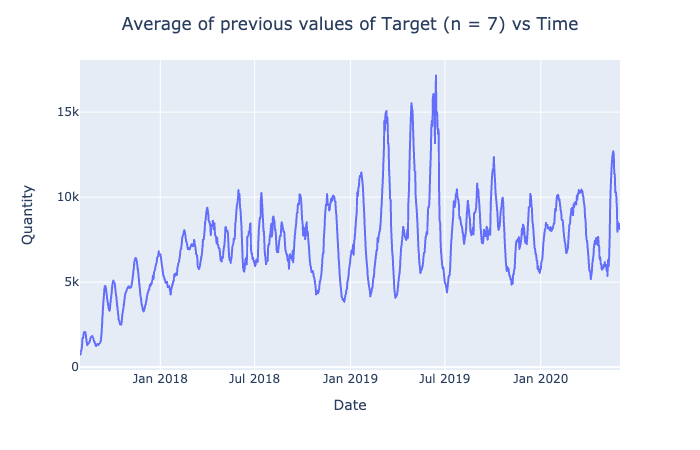
px.line(df, x = 'Date', y = n_prev_func(target.tolist(), 7, st.mean))\
.update_layout(title = "Average of previous values of Target (n = 7) vs Time",
title_x = 0.5,
yaxis_title = "Quantity").show()
target_smooth = pd.Series(n_prev_func(target.tolist(), 7, st.mean))
target_smooth
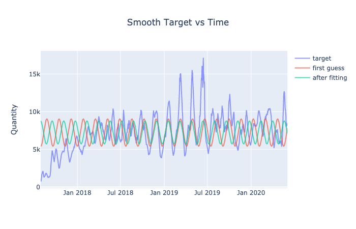
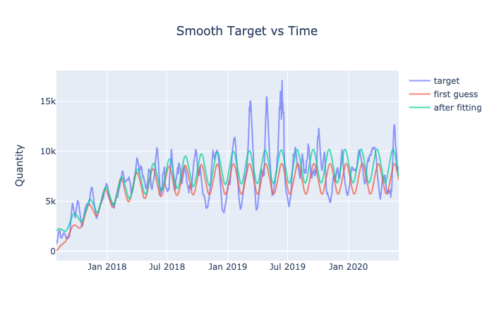
The following cell attempts to mathematically fit a curve that would represent the patterns in the data.
Refer to the following links for graphs:
import numpy as np
import plotly.graph_objects as go
from scipy.optimize import leastsq
from sklearn.metrics import r2_score

t = df.index
data = target_smooth # any target can be used here
date = df['Date']


def fit_sin(x, params):
    # f(x) = a * sin(bx + c) + d
    assert len(params) == 4
    return params[0] * np.sin(params[1] * x + params[2]) + params[3]


def fit_sin_log(x, params):
    # g(x) = a / (1 + e^(bx)) + d
    # s(x) = g(x) * f(x)
    assert len(params) == 4 + 3
    return (params[0] / (1 + np.exp(params[1] * x)) + params[2]) * fit_sin(x, params[3:])


# returns the optimized parameters and the data of the model for given x
# by optimizing fitting and optimizing given function to the given data
def optimize(x, params, func, data, display_graph = False):
    data_guess = func(x, params)
    optimize_func = lambda var: (func(x, var) - data)**2
    params_opt = leastsq(optimize_func, params)[0]
    data_opt = func(x, params_opt)
    if display_graph == True:
        go.Figure()\
        .add_trace(go.Scatter(x = date,
                              y = data,
                              mode = 'lines',
                              name = 'target',
                              opacity = 0.7))\
        .add_trace(go.Scatter(x = date,
                              y = data_guess,
                              mode = 'lines',
                              name = 'first guess',
                              opacity = 0.7))\
        .add_trace(go.Scatter(x = date,
                              y = data_opt,
                              mode = 'lines',
                              name = 'after fitting',
                              opacity = 0.7))\
        .update_layout(title = "Smooth Target vs Time",
                   title_x = 0.5,
                   yaxis_title = "Quantity").show()
    return params_opt, data_opt


# guess parameters for sin and optimize
params = [st.mean(data) / 4,
          2 * np.pi / (558 - 507),
          545,
          st.mean(data)]
results_sin = optimize(t, params, fit_sin, data, display_graph = True)


# guess parameters for logistical function and optimize
params = [2, -0.012, -1]
params.extend(results_sin[0])
results_sl = optimize(t, params, fit_sin_log, data, display_graph = True)

str_summary = 'Optimized parameters P for model: \nsl(x) = (P_1 / (1 + e^(P_2 * x)) + P_3) * (P_4 * sin(P_5 * x + P_6) + P_7)'
for i in range(0, len(results_sl[0])):
      str_summary += '\n\t\tP_' +  str(i + 1) + ' = ' + str(round(results_sl[0][i], 4))
str_summary += '\n\nVariance explained by the model: ' + str(round(r2_score(target_smooth, results_sl[1]),4))
print(str_summary)
Assuming that the target variable follows this exact model, we can identify another target variable, which is the error between the fitted model and the actual data. If our prediction models find the relationship between the features and error of this model, we will be able to predict the actual target. Se the following link for the graph:
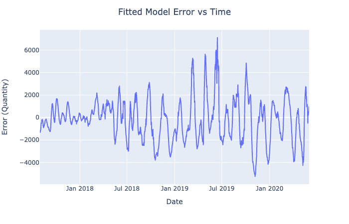
target_dif = data - results_sl[1]
px.line(df, x = 'Date', y = target_dif)\
.update_layout(title = "Fitted Model Error vs Time",
               title_x = 0.5,
               yaxis_title = "Error (Quantity)").show()

target_dif
Preprocessing and Training/Test Selection and Feature Selection
We created an object Split to keep track of our splitted, scaled, and selected sets better. The object is initialized with features target and a name. It has functions that scales X sets selects features.
import math
from sklearn.feature_selection import RFE
from sklearn.preprocessing import MinMaxScaler
from sklearn.model_selection import train_test_split
from sklearn.tree import DecisionTreeRegressor

# class that represents a training/testing split of features and targets
class Split:

    # constructor
    def __init__(self, features, target, name):
        self.features, self.target, self.name = features, target, name
        self.num_features = len(features.columns)
        self.X_train, self.X_test, self.y_train, self.y_test = train_test_split(features, target, random_state = 3000)
        self.selected_features = []

    # scale X sets
    def scale_test_sets(self):
        # create scaler object based on X_train
        scaler = MinMaxScaler().fit(self.X_train)
        # scale X train and test sets
        self.X_train_scaled = scaler.transform(self.X_train)
        self.X_test_scaled = scaler.transform(self.X_test)
        # assing selected sets to scales X train and test sets
        self.X_train_selected = self.X_train_scaled
        self.X_test_selected = self.X_test_scaled

    # define selected features
    def select_features(self, num_features = None):
        # defualt number of features to select is the square root of the current number of features + 1
        if num_features == None:
            num_features = math.floor(math.sqrt(self.num_features)) + 1
        # instantiate selection object
        feature_selection = RFE(DecisionTreeRegressor(random_state = 3000), n_features_to_select = num_features)
        # fit scaled X train set to y train set
        feature_selection.fit(self.X_train_scaled, self.y_train)
        # transform previous scaled sets and assign them to selected
        self.X_train_selected = feature_selection.transform(self.X_train_scaled)
        self.X_test_selected = feature_selection.transform(self.X_test_scaled)

        # print selected feature names
        out = 'Selected features for ' + self.name + ':\n'
        for feature in [feature for feature, status in zip(self.features, feature_selection.get_support()) if status == True]:
            out += '\t' + feature + '\n'
            self.selected_features.append(feature)
        print(out + '\n')


# list of different Split objects
splits = [Split(features, target, 'Features and target'),
          Split(features, target_smooth, 'Features and smoothed target'),
          Split(features, target_dif, 'Features and Fitted Error'),
          Split(features_combined, target, 'Features Combined and target'),
          Split(features_combined, target_smooth, 'Features Combined and smoothed target'),
          Split(features_combined, target_dif, 'Features Combined and Fitted Error')]

# scale training sets and select features for each Split
for split in splits:
    split.scale_test_sets()
    split.select_features()
3.2. Data Exploration
The following data exploration is only going to cover the data we identified as significant. First, we will explore the relationship between the selected features in one of our splits and then explore the correlations between features and the target variable.
import matplotlib.pyplot as plt
import seaborn as sns

# enable in-line rendering
%matplotlib notebook

# construct the data frame of the selected features for fifth split and add a produced column
heat_df = features_combined[splits[4].selected_features]
heat_df['Produced'] = target_smooth
plt.rcParams.update({'font.size': 7})
plt.figure(figsize=(10, 10))
sns.heatmap(heat_df.corr(), cmap='coolwarm', square = True)
plt.savefig("heatmap.png")

Visualization Explanation - Heatmap
Please see the heatmap image here:
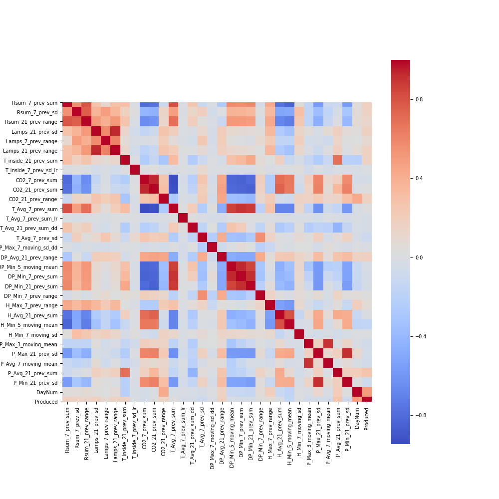
This heatmap shows the correlations between the selected features in split "Features Combined and smoothed target" and smooth target. As can be seen on the graph, there is no strong linear correlation between the smooth target and the selected features. This is somewhat reasonable given the nonlinear nature of our data. More importantly, we suspect that our target variable is going to be affected by a combination of these selected features. The only strong correlation appears to be between similar selected features for obvious reasons. On the graph, they can be seen as rectangles of the same color.
for feature in ['Rsum', 'Lamps', 'T_inside', 'H_Avg']:
    px.scatter(df,
               x = feature,
               y = target_dif,
               template = 'none',
               color = target_dif,
               opacity = 0.8,
               trendline = 'ols')\
    .update_traces(marker={"size":7})\
    .update_layout(title = "Error vs " + feature,
                   title_x = 0.5,
                   yaxis_title = "Fitted Error (Quantity)")\
    .show()
Visualization Explanation - Scatter Plots
Please see the scatter plots here:
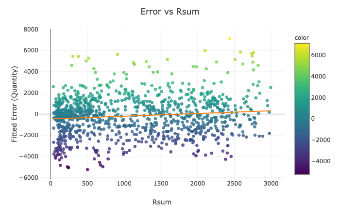
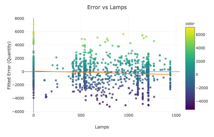
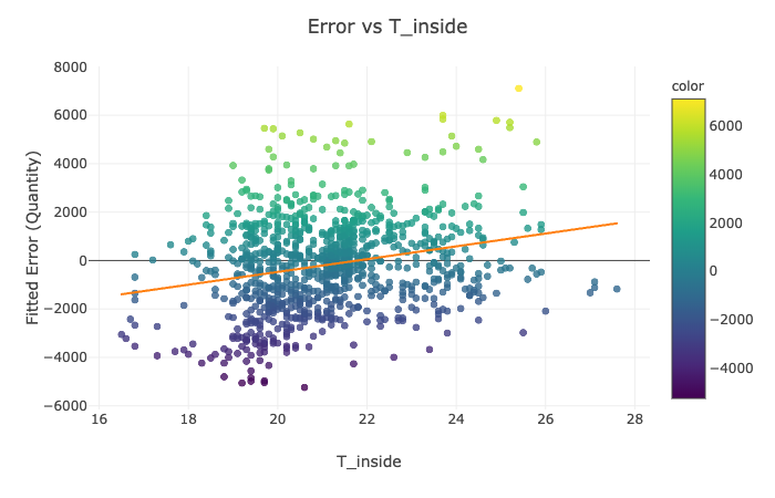
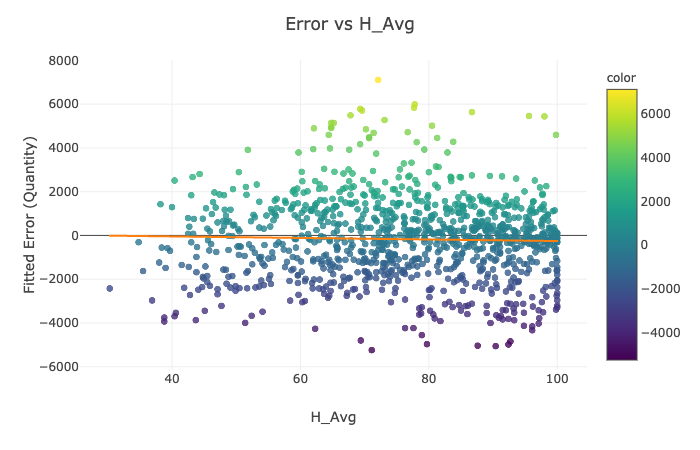
In Figures 1-4, we plot the selected features of the third split against the fitted mathematical model's error and display the ordinary least squares line. On all of the above graphs besides T_inside, we observe a zero correlation, which makes sense due to the sinusoidal nature of our data. The points are evenly distributed on top and the bottom of the zero line and, hence, cancel each other out. The only significant positive correlation is present on the plot of Error vs. T_inside. If you look at the earlier graph called 'Fitted Model Error vs. Time,' you can observe that most positive errors occur in the summer, while most negative errors occur in the winter. Similarly, the temperature tends to be higher in the summer and colder in the winter. Hence, these two variables are very likely to correlate.
3.3. Model Construction
Based on the observations made from the visualizations above, we suspect there will be a relationship between the target variables and the selected mathematically summarized weather conditions.
# model dictionary
from sklearn.svm import LinearSVR
from sklearn.neighbors import KNeighborsRegressor
from sklearn.kernel_ridge import KernelRidge
from sklearn.linear_model import Ridge
from sklearn.linear_model import Lasso
from sklearn.linear_model import BayesianRidge
from sklearn.linear_model import LinearRegression
from sklearn.gaussian_process import GaussianProcessRegressor

estimators = {'Linear': LinearRegression(),
              'Ridge': Ridge(max_iter = 100000),
              'Lasso': Lasso(max_iter = 100000),
              'kNN': KNeighborsRegressor(),
              'BayesianRidge': BayesianRidge(n_iter = 100000),
              'KernelRidge': KernelRidge(),
              'GaussianProcess': GaussianProcessRegressor()}

estimators.values()
def fit_regressors(estimators, split):

    X_train, X_test, y_train, y_test = split.X_train_selected, split.X_test_selected, split.y_train, split.y_test

    # select a classifier and change parameters
    for name, estimator in estimators.items():

        # fit a model to the training data
        estimator.fit(X = X_train, y = y_train)

        # compute R^2 scores
        train_score = round(r2_score(y_train, estimator.predict(X_train)), 4)
        test_score = round(r2_score(y_test, estimator.predict(X_test)), 4)

        #print accuracy
        print(name, ':\n\tR^2 value for training set: ', train_score,
              '\n\tR^2 value for testing set : ', test_score, '\n', sep = '')


for split in splits:
    print('–––––––––––––––––––––––––––––––––––––––––––––––––\n\n\t\t' + split.name.upper()  + '\n')
    fit_regressors(estimators, split)
3.4. Model Evaluation
We discarded innefective models and decided to evaluate those with a passable performance using the following
Predicting Smoothed Target
- Linear for features combined with smoothed target
- KNN for features combined with smoothed target
- Gaussian for features combined with smoothed target
Predicting Fitted Error
- Linear for features combined and fitted error
- KNN for features combined with smoothed target
- Guassiann for features combiend with smoothed target
Evaluation Metrics using Cross Validation
- R^2
- Mean Accuracy
- Standard Deviation
f_combined_smoothed = splits[4]
f_combined_smoothed_err = splits[5]
Cross validation of highest performing models on selected features for smoothed target and error
from sklearn.model_selection import KFold
kfold = KFold(n_splits = 10, random_state = 3000, shuffle = True)
from sklearn.model_selection import cross_val_score
from sklearn.linear_model import LinearRegression

evalEstimators = {'Linear': LinearRegression(),
              'kNN': KNeighborsRegressor(),
              'GaussianProcess': GaussianProcessRegressor()}

#Dictionary of model names and scores
scores_target_smoothed = {}
scores_error_smoothed = {}
for name, model in evalEstimators.items():
    scores_target_smoothed[name] = cross_val_score(estimator=model,X=f_combined_smoothed.X_train_selected,
                                                   y=f_combined_smoothed.y_train,cv = 5)
    print(name + " Target_Smoothed done")
    scores_error_smoothed[name] = cross_val_score(estimator=model,X=f_combined_smoothed_err.X_train_selected,
                                                  y=f_combined_smoothed_err.y_train,cv = 5)
    print(name + " Error Fitted done")
Prediction Accuracy
- KNN and Gaussian appear to have the best predictive performance on the validation tests
- The same is true when predicting Error CV mean scores
- Low standard deviations indicate that the afforementioned models are reliably accurate
print("Target Smoothed CV scores")
for name, score in scores_target_smoothed.items():
    print('–––––––––––––––––––––––––––––––––––––––––––––––––\n\n\t\t' + name  + '\n')
    print("Mean Score:",score.mean())
    print("Standard Deviation",f"{score.std():.2%}")
print("\n\n")
print("\t\tError CV Mean Scores")
for name, score in scores_target_smoothed.items():
    print('–––––––––––––––––––––––––––––––––––––––––––––––––\n\n\t\t' + name  + '\n')
    print("Mean Score:",score.mean())
    print("Standard Deviation",f"{score.std():.2%}")
3.5. Model Optimization
Rationale For Tuning
After performing a cross-validation test to evaluate our three best models, we can then select from that set, two models: kNN and Gaussian Process for hyper-parameter tuning. Since these models have a high degree of accuracy, we want to reduce the risk of over-fitting these models to retain predictive value upon future data for flower production.
Tuning
from sklearn.model_selection import train_test_split
from sklearn.model_selection import GridSearchCV

param_grid1 = {'alpha':[.001, .01, .1, 1, 10, 100]}
param_grid2 = {"n_neighbors":[1, 2, 3, 5, 10], "metric": ["euclidean", "manhattan", "minkowski"]}
best_estimators = {
              'kNN': KNeighborsRegressor(),
              'GaussianProcess': GaussianProcessRegressor()}

def optimize(x_train, y_train):
    out = {}
    for name, model in best_estimators.items():
        if name == 'kNN':
            grid_search = GridSearchCV(model, param_grid2, cv=5)
        if name == 'GaussianProcess':
            grid_search = GridSearchCV(model, param_grid1, cv=5)
        grid_search.fit(X=x_train, y=y_train)
        print(name)
        print("\tBest cross-validation score: ", grid_search.best_score_)
        print("\tBest parameters: ", grid_search.best_params_)
        print()
        out[name] = grid_search.best_params_
    return out
Results on Training Set For Parameter Tuning
print("Model Optimization for Selected features on Smoothed Target data \n__________________________________________________ \n")
best_params = optimize(f_combined_smoothed.X_train_selected, f_combined_smoothed.y_train)
print('\n')
print("Model Optimization for selected features for error prediction \n__________________________________________________ \n")
best_params_error = optimize(f_combined_smoothed_err.X_train_selected, f_combined_smoothed_err.y_train)
print('\n')
3.6. Model Testing
Using our findings from the parameter tuning phase, we will test the accuracy and performance of our models on our testing data set
param_grid1 = {'alpha':[.001, .01, .1, 1, 10, 100]}
param_grid2 = {"n_neighbors":[1, 2, 3, 5, 10], "metric": ["euclidean", "manhattan", "minkowski"]}
optimal_estimators = {
              'kNN Smoothed Target': KNeighborsRegressor(n_neighbors = 1, metric = 'manhattan'),
              'GaussianProcess Smoothed Target': GaussianProcessRegressor(alpha = .001),
                'kNN Error' : KNeighborsRegressor(n_neighbors = 2),
                'GaussianProcess Error' :GaussianProcessRegressor(alpha = .001) }

# selected on smooth and error
for split in splits[4:]:
    print('–––––––––––––––––––––––––––––––––––––––––––––––––\n\n\t\t' + split.name.upper()  + '\n')
    fit_regressors(optimal_estimators, split)
4. DISCUSSION
Summary of Analysis
In order to perform our analysis, we split our weather conditions and greenhouse data into feature variables and target variable, the number of flowers produced. Then we created several functions like sum, range, or standard deviation that were applied to every feature and recorder in a 'features combined' data frame along with making our features polynomial to explore nonlinear relationships. We also smoothened our target variable and tried to come up with a mathematical model describing its distribution. As a result, we obtained two additional targets (smoothened amount of flowers produced and the error between the mathematical model and the smoothened quantity produced) to explore in our data analysis. We did not visualize all of our data because of the sinusoidal nature of our target variable but focused on the selected relationships among our features and features with the number of flowers produced.
To run our regression models, we created six splits of data with a different combination of features and target variables (features, features combined, target, smooth target, error), scaled the appropriate sets, and selected the most significant features. We evaluated seven different supervised machine learning models - subcategory regression - using all six of the training and testing sets described previously. f We then evaluated the regression models using a cross validation split in order to adaquetely determine which models were the most promising and warranted hyper-parameter tuning. Our results dicated that kNN and Gaussian Process were our best models from the cross mean validation scores which were: 84% and 90% respectively.
Afterwards, we applied a GridSearchCV to fine tune the following parameters:
Smoothed Target Value
- Gaussian Process: Alpha Value = .001
- kNN: n_neighbors = 2 and Metric = Manhattan
Error Prediction
- Gaussian Process: Alpha Value = .001
- kNN: n_neighbors = 1 and Metric = Manhattan
Interpretation of Findings
Algorithms Compared
We compared Multiple Linear, Ridge, Lasso, kNN, BayesianRidge, KernelRidge, and GaussianProcess regression algorithms.
Algorithms with Best Performance The algorithms with the best performance were kNN and Gaussian process, and Linear Regression
Smoothed Target Value r^2
* Multiple Linear: 0.40
* kNN: .84
* Gaussian Process: .90

Error Prediction r^2
* Multiple Linear: 0.40
* kNN: .84
* Gaussian Process: .90
Evaluation after Optimization
After tuning and optimization we saw a moderate improvement in the results. After optimization, we were unable to improve the linear regression model to a sufficient standard, and as such, it was discarded from our final analysis.
The accuracy of the models on our testing data improved to the following values.
Smoothed Target Value r^2
* kNN: .96
* Gaussian Process: .94

Error Prediction r^2
* kNN: .98
* Gaussian Process: .94
Algorithms for Use in Predictive Model
We expected Bayesian Ridge, KernelRidge, and Gaussian Process regression algorithms to work best because the examples in the scikit learn documentations suggests that they are good at predicting sinusoidal data. However, upon review of our results we found that Gaussian Process was the only model from our original predictions that produced sufficient results. Knn and Gaussian models form the best predictive models for our data set.
Our Original Research Questions
Is there a linear relationship between the weather conditions and the number of flowers produced? If not, what is the relationship?
In our data visualization and analysis, we found that there is no direct linear relationship between the weather conditions and the number of flowers produced. Moreover, the linear regression model proved to one of the least accurate when it came to predicting the number of flowers produced or the deviation from the assumed cycle.
Is there an accumulative or delayed effect of the weather conditions on the dependent variable? What is it?
When we applied the feature selection technique, we discovered that accumulative, delayed, and other mathematically modified features had a more significant effect on the dependent variable than the current weather conditions.
Is there a pattern in the number of flowers produced? What periods appear to be more stable or have less noise in the number of flowers produced? What parts of the natural cycle (amplitude, period, vertical shift) are affected by the weather?
It is evident from our visualizations and attempts to mathematically describe the pattern that the number of flowers produced follows a sinusoidal pattern.
Is there a relationship between the weather conditions and the deviation from the natural production cycle? Which features are the most influential on the deviations of the cycle?
We were able to construct an accurate model with the deviation from the cycle as a target variable, which means that there has to be a relationship. The list of significant features can be found in the data analysis section, but we are not sure about the order of significance. Coming up with twenty or so selected features has proven to be very computationally expensive for the combined dataset.
Is there a linear or nonlinear regression model that can predict the number of flowers produced? Which one is more accurate?
Yes. kNN (non linear) and Gaussian Process were both predictive of our data. However, neither of those models are linear.
How do the features correlate with each other? Can we reduce their number to make the prediction model more accurate?
In the heat map visualization of our data, we found that the most significant features do not correlate with each other. However, we did not check all the features, and the ones we have already been selected as significant. Reducing the number of features in the combined data set proved to produce more accurate prediction models and less accurate predictive models for an original data set of features.
Reflection on Our Findings
In our original problem, we wanted to find out if our selected (strongly correlated) wheather conditions were predictive of the sinusoidal pattern originally observed in our data. After testing a variety of models including several linear models and kNN and Gaussian Process we found that linear models were not predictive of our data but kNN and Gaussian Process models were. Upon tuning the parameters of our models and employing our feature selection, we were able to generate two highly accurate models that performed well under cross validation tests.
Conclusion
We expected better results from the Kernel Ridge regression as scikit learn documentation says it is often highly predictive of sinusoidal data. Perhaps we could have done a better job fine tuning the prameters of that specific model or perhaps a Kernel ridge regression warrants a more specific feature selection process. We were surprised that kNN model could be tuned to such a high degree of accuracy. The performance of the Gaussian Process was not surprising as it is often highly predictive of cyclical data.
Future work of this project could involve combining the error prediction model with the smoothed target prediction. Additionally we believe this model has effective real world utility for greenhouse companies and possibly for other crops that are farmed. The real world implications of this project could perhaps be employed by certain hedge funds or investment firms to predict yields of various crops (other than flowers) in order to effectively price commodity futures.
CONTRIBUTIONS
Jake:
- problem description and specification
- data acquisition
- feature and target extraction
- preprocessing and feature selection
- data exploration
Pranav
- Model Fitting and Selection
- Model Prediction
- Model Optimization
- Model Evaluation
- Model Testing